Hubbard model with FNQS#
This tutorial shows how to extend the Foundation NQS framework to fermionic systems. We
train a single network \(\psi(\sigma; U)\) simultaneously over a family of
1D Hubbard Hamiltonians parameterised by the on-site interaction \(U\).
The fermionic operators create, destroy, and number from
netket_foundation.operator are used to build the Hamiltonian, and
a backflow–Jastrow ansatz replaces the spin ViT used in Tutorial 1.
This tutorial covers:
Building the Hubbard Hamiltonian with
create(),destroy(),number()Constructing a fermionic FNQS with a ViT backflow and a multiplicative Jastrow factor
Training with
VMC_SRacross the full \(U\) range in one runComparing the resulting ground-state energies to exact diagonalisation
Quantum Fisher information \(\chi(U)\) via importance-sampling reweighting
For the spin-system FNQS workflow see Tutorial 1 – FNQS training basics. For the IS theory and the ESS diagnostic see Tutorial 3 – Importance Sampling.
∣NK⟩ Tip: HDF5Log/MLFlowLog/TensorBoardLog accept metadata={'L': 20, 'model': 'RBM'} to store hyperparameters with
the run.
System: 1D Hubbard chain#
with \(L = 8\) sites, periodic boundary conditions, \(t = 1\), half-filling (\(N_\uparrow = N_\downarrow = 4\)), and \(U \in [0, 4]\). At \(U = 0\) the system is a free Fermi gas; as \(U\) grows correlations build up and the Mott insulating regime is approached.
The Hubbard Hamiltonian is built using the second-quantisation operators
from netket_foundation.operator. The spin projections are encoded as
\(\uparrow \equiv +1\) and \(\downarrow \equiv -1\).
L         = 8
N_fermions = L // 2          # half-filling: 2 electrons per spin sector
graph      = nk.graph.Chain(L, pbc=True)
hi         = nk.hilbert.SpinOrbitalFermions(
    L, s=1/2, n_fermions_per_spin=(N_fermions, N_fermions)
)

ps = nkf.ParameterSpace(N=1, min=0.0, max=4.0)

up, down   = +1, -1
bonds_nn   = [tuple(e) for e in graph.edges()]

def create_operator(params):
    assert params.shape == (1,)
    U = params[0]
    t = 1.0
    H_t = sum(
        (
            fcdag(hi, i, spin) @ fc(hi, j, spin)
            + fcdag(hi, j, spin) @ fc(hi, i, spin)
        )
        for i, j in bonds_nn
        for spin in (up, down)
    )
    H_U = sum(fnc(hi, i, up) @ fnc(hi, i, down) for i in range(L))
    return -t * H_t.to_jax_operator() + U * H_U.to_jax_operator()

ha_p = nkf.operator.ParametrizedOperator(hi, ps, create_operator)

print(f"Hilbert space: {hi}")
print(f"Number of basis states: {hi.n_states}")
print(f"U in [{ps._min}, {ps._max}]")
Hilbert space: SpinOrbitalFermions(n_orbitals=8, s=1/2, n_fermions=8, n_fermions_per_spin=(4, 4))
Number of basis states: 4900
U in [0.0, 4.0]
Fermionic FNQS architecture#
Spin systems use a plain ViT that maps occupation strings to log-amplitudes.
For fermions the ansatz must encode the correct antisymmetry.
We use a backflow + Jastrow architecture assembled by ViTFermionicFNQS():
ViT trunk — a translation-equivariant Vision Transformer that processes the occupation string (and the coupling \(U\)) into per-orbital features.
Backflow — wraps the ViT to produce the matrix elements of a (generalised) Slater determinant, giving the correct fermionic sign structure.
Jastrow MLP — a multiplicative correlator on top of the determinant that captures density–density correlations missed by the mean-field picture.
The full wavefunction is \(\psi = \psi_{\mathrm{Jastrow}} imes \psi_{\mathrm{backflow}}\),
with all derived dimensions (d_output, n_patches) computed automatically from
the Hilbert space and graph.
Both sub-networks receive \(U\) as an extra input through the shared
ParameterSpace, so a single set of weights
covers the entire \(U\) range.
pars_type = jnp.float64
seed      = 42

ma = ViTFermionicFNQS(
    hilbert=hi, graph=graph, n_coups=ps.size,
    num_layers=2, d_model=16, heads=2, b=2,
    param_dtype=pars_type,
)

# Replicas uniformly spaced across U ∈ [0, 4]
n_replicas      = 16
parameter_array = jnp.linspace(0.0, 4.0, n_replicas, dtype=pars_type).reshape(-1, 1)

sa = nk.sampler.MetropolisFermionHop(
    hilbert=hi, n_chains=n_replicas, graph=graph, sweep_size=hi.size
)
vs = nkf.FoundationalQuantumState(
    sa, ma, ps, n_replicas=n_replicas, seed=seed, n_samples=n_replicas * 32
)
vs.parameter_array = parameter_array

print(f"Parameters: {vs.n_parameters}")
print(f"Replicas:   {vs.n_replicas},  samples: {vs.n_samples}")
Parameters: 5520
Replicas:   16,  samples: 512
Training#
VMC_SR drives all replicas simultaneously.
We pass use_ntk=True to compute the natural gradient via the Neural
Tangent Kernel.
The learning rate follows a linear decay and the diagonal shift
decays exponentially to allow fine convergence in the final iterations.
epochs        = 512
optimizer     = optax.sgd(learning_rate=optax.linear_schedule(init_value=0.05, end_value=0.005, transition_steps=epochs))
diag_shift    = optax.exponential_decay(1e-2, end_value=1e-4, transition_steps=32, decay_rate=0.8)

gs = nkf.VMC_SR(
    ha_p,
    optimizer,
    variational_state=vs,
    diag_shift=diag_shift,
    use_ntk=True,
    linear_solver = nk.optimizer.solver.pinv_smooth(rtol=1e-8, rtol_smooth=1e-8)
)

t0 = time.perf_counter()
gs.run(epochs, show_progress=True)
print(f"Training done in {time.perf_counter() - t0:.0f} s")
online_statistics: chain_length=32, exponential moving average window: 50, decay=0.500
Training done in 165 s
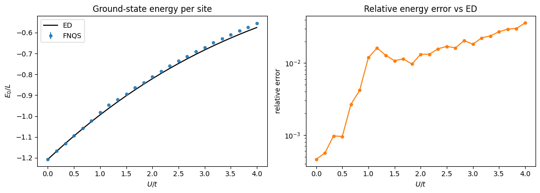
Post-training evaluation#
After training, vs.get_state(params) extracts a standard
netket.vqs.MCState pinned to a specific \(U\) value.
We sweep over the full \(U\) grid, measure the energy, and compare
it to exact diagonalisation (ED).
Because the Hilbert space is small (\(\dim = 4900\) at half-filling on \(L = 8\))
the ED reference is essentially instantaneous.
U_sweep = jnp.linspace(0.0, 4.0, 25)

# Exact diagonalisation reference
ed_E = np.array([
    nk.exact.lanczos_ed(create_operator(jnp.array([float(U)])), k=1, compute_eigenvectors=False).item()
    for U in U_sweep
])

# FNQS evaluation via fresh MCMC at each point
vmc_E     = []
vmc_E_err = []

for U in U_sweep:
    op = create_operator(jnp.array([float(U)]))
    mc = vs.get_state(jnp.array([float(U)]))
    mc.n_samples = 1024
    mc.thermalise(op, rhat_tol=1.03, verbose=False)   # converge the chains, R-hat < rhat_tol
    result = mc.expect(op)
    vmc_E.append(float(result.mean.real))
    vmc_E_err.append(float(result.error_of_mean))

vmc_E     = np.array(vmc_E)
vmc_E_err = np.array(vmc_E_err)

print("Evaluation done.")
print(f"Max relative error: {np.max(np.abs((vmc_E - ed_E) / ed_E)):.4f}")
Evaluation done.
Max relative error: 0.0362
fig, axes = plt.subplots(1, 2, figsize=(11, 4))

# Left: ground-state energy vs U
ax = axes[0]
ax.plot(U_sweep, ed_E / L, "k-", lw=1.5, label="ED")
ax.errorbar(
    U_sweep, vmc_E / L, yerr=vmc_E_err / L,
    fmt="o", ms=4, color="tab:blue", label="FNQS", alpha=0.85,
)
ax.set_xlabel("$U/t$")
ax.set_ylabel("$E_0 / L$")
ax.set_title("Ground-state energy per site")
ax.legend()

# Right: relative error vs U
ax = axes[1]
rel_err = np.abs((vmc_E - ed_E) / np.abs(ed_E))
ax.plot(U_sweep, rel_err, "-o", ms=4, color="tab:orange")
ax.set_xlabel("$U/t$")
ax.set_ylabel("relative error")
ax.set_title("Relative energy error vs ED")
ax.set_yscale("log")

plt.tight_layout()
plt.show()
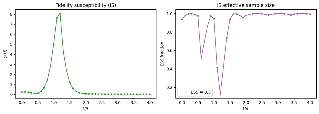
Quantum Fisher information via IS#
The fidelity susceptibility with respect to \(U\) is
It measures how rapidly the ground-state manifold changes as \(U\) is varied:
a large \(\chi\) signals that the wavefunction is highly sensitive to the
interaction strength, which typically happens near crossover or transition
points.
We compute it via IS: reuse the nearest anchor state’s samples with IS weights,
then evaluate the weighted variance of \(\partial_U\log\psi\) using jax.jacfwd.
U_anchors = np.linspace(0.25, 3.75, 6)
U_qfi     = np.linspace(0.0,  4.0,  41)

# Build anchor MCStates with more samples for reliable IS weights, thermalising
# each one (MCMC until R-hat < rhat_tol) before it is used as an IS reference.
anchor_states = {}
for U0 in U_anchors:
    mc = vs.get_state(jnp.array([float(U0)]))
    mc.n_samples = 2048
    mc.thermalise(create_operator(jnp.array([float(U0)])), rhat_tol=1.03, verbose=False)
    anchor_states[U0] = mc

def nearest_anchor(U):
    return U_anchors[np.argmin(np.abs(U_anchors - U))]

# IS sweep for chi(U)
qfi_vals = []
qfi_ess  = []

for U0 in U_qfi:
    mc_ref = anchor_states[nearest_anchor(U0)]
    pars   = jnp.array([float(U0)])
    is_st  = ISState.from_mc_state(mc_ref, pars)
    result = is_st.expect(SusceptibilityObservable(hi))
    qfi_vals.append(float(result.mean[0, 0]))
    qfi_ess.append(is_st.ess_fraction)

qfi_vals = np.array(qfi_vals)
qfi_ess  = np.array(qfi_ess)

print(f"QFI sweep done. Peak at U = {U_qfi[np.argmax(qfi_vals)]:.2f}")
print(f"Min ESS fraction: {qfi_ess.min():.2f}")
QFI sweep done. Peak at U = 1.20
Min ESS fraction: 0.13
fig, axes = plt.subplots(1, 2, figsize=(11, 4))

ax = axes[0]
ax.plot(U_qfi, qfi_vals, "-o", ms=3, color="tab:green")
ax.set_xlabel("$U/t$")
ax.set_ylabel(r"$\chi(U)$")
ax.set_title("Fidelity susceptibility (IS)")

ax = axes[1]
ax.plot(U_qfi, qfi_ess, "-o", ms=3, color="tab:purple")
ax.axhline(0.3, ls="--", color="gray", lw=0.8, label="ESS = 0.3")
ax.set_xlabel("$U/t$")
ax.set_ylabel("ESS fraction")
ax.set_title("IS effective sample size")
ax.legend()

plt.tight_layout()
plt.show()