Importance Sampling for observable estimation

Importance Sampling for observable estimation#

In Variational Monte Carlo (VMC) we estimate expectation values with statistical averages

\[ \langle O \rangle_\psi = \frac{\langle \psi | \hat O | \psi\rangle}{\langle \psi | \psi \rangle} \approx \frac{1}{N_s} \sum_{i=1}^{N_s} O_\text{loc}(\sigma_i), \qquad O_\text{loc}(\sigma) = \sum_\eta \langle\sigma|\hat O|\eta\rangle \frac{\psi(\eta)}{\psi(\sigma)}, \]

where \(p(\sigma) = |\psi(\sigma)|^2 / \lVert\psi\rVert^2\) is the Born probability from which the samples \(\{\sigma_i\}_{i=1}^{N_s}\) are drawn, \(\sigma_i \sim p(\sigma)\).

Sampling is a bottleneck for Foundation NQS

After optimization on \(H(\lambda)\), the Foundation NQS provides parameters for \(\psi(\sigma; \lambda)\) across the full parameter range. But computing observables at a given \(\lambda_0\) requires extracting \(\psi(\sigma; \lambda_0)\) and thermalizing the corresponding MCMC chains. When performing fine sweeps, or probing high-dimensional parameter spaces, or performing extensive disorder averages, this can quickly become extremely expensive.

In particular, values of the parameters \(\lambda_0\) close by will give nearly identical \(|\psi(\sigma; \lambda_0)|^2\), so rethermalising the chains from scratch is probably wasteful.

A natural fix is reweighting via importance sampling, which we discuss below.

Reweighting identity and Effective Sample Size (ESS)#

We want to estimate \(\langle O\rangle\) for a target state \(\psi_\text{tgt}\), but we only have samples \(\{\sigma_i\}\) drawn from a reference state \(\psi_\text{ref}\). Defining the weights

\[ w_i = \frac{|\psi_\text{tgt}(\sigma_i)|^2}{|\psi_\text{ref}(\sigma_i)|^2}, \]

a few lines of algebra give the self-normalized IS estimator:

\[ \widehat{\langle O\rangle}_\text{tgt} = \frac{\sum_i w_i\, O_\text{loc}^\text{tgt}(\sigma_i)}{\sum_i w_i}. \]

The standard diagnostic for IS quality is the Effective Sample Size:

\[ \text{ESS} = \frac{\left(\sum_i w_i\right)^2}{\sum_i w_i^2}, \qquad 1 \le \text{ESS} \le N, \]

i.e. the number of equally-weighted samples that would give the same statistical power as the \(N\) unevenly-weighted ones.

The key insight is that an \(\text{ESS} < N\) corresponds to a bias in the MC estimator. The farther that \(\text{ESS}/N\) is from 1, the more biased the estimator is.

ESS / N	Meaning
\(\approx 1\)	All weights equal (\(\psi_\text{tgt} = \psi_\text{ref}\)). Perfect reuse.
\(\gtrsim 0.1\)	Reasonable overlap. The Importance sampling estimate is trustworthy.
\(\lesssim 0.01\)	A few samples dominate. Estimator is degenerate and is biased.

ISState.expect reports \(\sigma_{\bar O} = \sqrt{\mathrm{Var}_w(O_\text{loc}) / \text{ESS}}\), so a collapsing ESS inflates the error bar accordingly.

Example: fine sweep for the transverse-field Ising chain#

We train a small Foundation NQS for the one-dimensional transverse-field Ising model across a range of transverse fields \(h\), pick a few anchor points, and produce a fine sweep by reweighting.

∣NK⟩ Tip: To make sure your Markov chains are well-mixed, call vstate.thermalise(H) after loading a checkpoint.

The one-dimensional transverse-field Ising model on \(L=10\) spins with periodic boundary conditions has the following hamiltonian:

\[ \hat H(h_0) = -\sum_{i=1}^L \sigma^z_i \sigma^z_{i+1} - h_0 \sum_{i=1}^L \sigma^x_i. \]

where \(\sigma^\alpha_{L+i} = \sigma^\alpha_{i}\) for \(\alpha \in [x,y,z]\) and \(i=1,...,L\)

System: 1D Ising, L=10, h0 in [0.75, 2.0]

Training of the Foundational NQS#

We use a small ViTFNQS trained with the natural-gradient VMC driver across 8 replicas, each at a different \(h_0\) uniformly spaced in \([0.75, 2.0]\).

online_statistics: chain_length=4, exponential moving average window: 50, decay=0.920

Training done in 127 s

Anchor points#

We pick 7 anchor points evenly spaced in \([0.8, 1.9]\) and run full MCMC at each one. These will be the reference states for IS. All other \(h_0\) values in the fine sweep will borrow samples from their nearest anchor.

For each anchor we call vs.get_state(h0) to get the parameters for the state at the transverse field \(h_0\), then we draw a fresh batch of MCMC samples.

# Anchor h0 values where we do full MCMC.
h_anchors = np.linspace(0.8, 1.9, 7)

# Fine sweep: 51 points across the full range.
h_sweep = np.linspace(0.75, 2.0, 51)

# Build and thermalise the anchor MCStates. `thermalise` runs MCMC until the
# chains are converged (Gelman-Rubin R-hat below `rhat_tol`); a fixed number of
# manual `.sample()` calls would give no such guarantee, and reusing an
# un-thermalised reference would bias every IS estimate downstream.
anchor_states = {}
for h0 in h_anchors:
    pars = jnp.array([h0])
    vs_reference = vs.get_state(pars)
    vs_reference.n_samples = 4096  # more samples for the final evaluation
    vs_reference.thermalise(create_operator(pars), rhat_tol=1.03, verbose=False)
    anchor_states[h0] = vs_reference
    print(f"  anchor h0={h0:.2f}  samples: {vs_reference.samples.shape}")

def nearest_anchor(h, anchors=h_anchors):
    """Return the anchor h0 closest to h."""
    return anchors[np.argmin(np.abs(anchors - h))]

  anchor h0=0.80  samples: (256, 16, 10)

  anchor h0=0.98  samples: (256, 16, 10)

  anchor h0=1.17  samples: (256, 16, 10)

  anchor h0=1.35  samples: (256, 16, 10)

  anchor h0=1.53  samples: (256, 16, 10)

  anchor h0=1.72  samples: (256, 16, 10)

  anchor h0=1.90  samples: (256, 16, 10)

Two ways to build an importance-sampled state#

NetKet foundation gives you two equivalent ways to construct the importance-sampled state. Both take a reference (an already-thermalised distribution) and a target set of parameters, and both reuse the reference samples to estimate observables at the target — they differ only in where the reference lives.

1. In memory, from an MCState — quickest when the reference state is already in memory:

is_st = ISState.from_mc_state(mc_ref, pars)

2. From a reference saved to disk — the reference distribution (physical samples + log-probabilities) is bundled into a lightweight SamplesWithProb object that you can save once and reload later:

nkf.vqs.samples_with_probability(mc_ref).save("anchor")          # once, after thermalising
reference = nkf.expectation_value.SamplesWithProb.load("anchor")  # later, in any analysis script
is_st = vs.is_state(pars, reference=reference)

We recommend the disk-based route for real workflows. Thermalising the anchor chains is by far the most expensive step; saving the reference once lets you re-run the (cheap) analysis as many times as you want — new observables, finer grids, a separate notebook or script — without ever resampling. The in-memory form is used in the rest of this notebook only to keep the example self-contained.

The cell below shows that the two routes give the same estimate:

# The two routes produce the same ISState. We demonstrate this on a single
# anchor, targeting a nearby field value h0.
mc_ref = anchor_states[h_anchors[1]]   # an already-thermalised reference state
pars   = jnp.array([1.0])              # target parameters

# Route 1 — in memory, straight from the sampled MCState.
is_mem = ISState.from_mc_state(mc_ref, pars)

# Route 2 — persist the reference to disk, then rebuild from the saved bundle.
nkf.vqs.samples_with_probability(mc_ref).save("anchor_ref")          # writes anchor_ref.npz
reference = nkf.expectation_value.SamplesWithProb.load("anchor_ref")
is_disk = vs.is_state(pars, reference=reference)

E_mem  = is_mem.expect(create_operator(pars)).mean.real
E_disk = is_disk.expect(create_operator(pars)).mean.real
print(f"in-memory : E = {E_mem:.6f}")
print(f"from disk : E = {E_disk:.6f}")

in-memory : E = -12.784639
from disk : E = -12.784639

For each \(h_0\) in the fine sweep we:

Find the nearest anchor.
Build an ISState from the anchor reference and the target variables via ISState.from_mc_state(mc_ref, pars).
Call .expect(H) and .expect(Mz2) on the same ISState — IS weights are computed once and reused for both estimators.

# --- warm-up: compile one throwaway call per anchor ---
for h0, mc in anchor_states.items():
    _is = ISState.from_mc_state(mc, jnp.array([h0]))
    jax.block_until_ready(_is.expect(create_operator(jnp.array([h0]))).mean)

is_E, is_E_err, is_Mz2, is_Mz2_err = [], [], [], []
is_ess_frac, is_anchor_used = [], []

for h0 in h_sweep:
    # 1. Nearest anchor
    h_anc  = nearest_anchor(h0)
    mc_ref = anchor_states[h_anc]
    pars   = jnp.array([h0])

    # 2. ISState — weights computed once, shared across all estimators below
    is_st = ISState.from_mc_state(mc_ref, pars)

    # 3. IS estimates (cached weights reused automatically)
    r_E   = is_st.expect(create_operator(pars))
    r_Mz2 = is_st.expect(Mz2)

    is_E.append(float(r_E.mean.real))
    is_E_err.append(float(r_E.error_of_mean))
    is_Mz2.append(float(r_Mz2.mean.real))
    is_Mz2_err.append(float(r_Mz2.error_of_mean))
    is_ess_frac.append(is_st.ess_fraction)
    is_anchor_used.append(h_anc)

print(f"IS sweep done ({len(h_sweep)} points, {len(h_anchors)} anchors).")

IS sweep done (51 points, 7 anchors).

Baseline: full MCMC at every point#

For comparison, we now do what one would do without IS: for each \(h_0\) in the same sweep, call vs.get_state(h0), run full MCMC, and compute observables with MCState.expect.

Baseline sweep done (51 points).

Exact diagonalisation (ground truth)#

Since \(L=10\) is small enough for exact diagonalisation, we compute the exact ground-state energy and \(\langle M_z^2\rangle\) across the sweep for comparison.

Exact diagonalisation done.

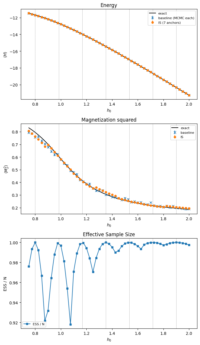
Comparison plots#

Here we show three panels with the following plots

Energy \(\langle H\rangle\) vs \(h_0\): exact (line), baseline (crosses), IS (circles with error bars).
Magnetization \(\langle M_z^2\rangle\) vs \(h_0\)
ESS / N vs \(h_0\): the IS quality diagnostic.

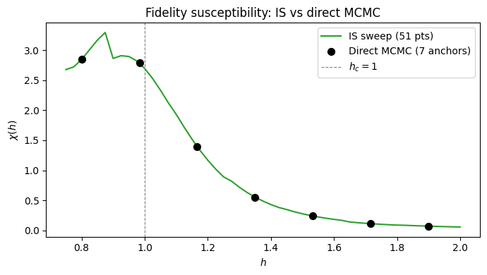
../_images/78514f271998cefc44f19ea7a85eb5bd6fa35a05a298601eadec6294a10a021a.png

Quantum Fisher information: IS vs direct MCMC#

The fidelity susceptibility with respect to \(h\),

\[ \chi(h) = \mathrm{Var}_{|\psi(h)|^2}\!\left[\partial_h \log\psi(\sigma;\,h)\right], \]

peaks at the quantum phase transition \(h_c = 1\).

Below we show two ways to evaluate it, both through the SusceptibilityObservable:

Direct MCMC — call mc.expect(SusceptibilityObservable(hi)) on the 7 already-sampled anchor states. This returns a StatsBatch with .mean and .error_of_mean.
IS sweep — build ISState.from_mc_state(mc_ref, target_vars) for each \(h_0\), then call is_st.expect(SusceptibilityObservable(hi)). This reuses the anchor samples without performing the MCMC sampling again.

# Direct QFI at anchor points (reuses already-sampled states, no extra MCMC).
qfi_direct_h    = list(anchor_states.keys())
qfi_direct_vals = [float(mc.expect(SusceptibilityObservable(hi)).mean[0, 0])
                   for mc in anchor_states.values()]

# IS sweep over the fine grid (weights cached per ISState).
qfi_is_vals, qfi_is_ess = [], []
for h0 in h_sweep:
    pars   = jnp.array([h0])
    mc_ref = anchor_states[nearest_anchor(h0)]
    is_st  = ISState.from_mc_state(mc_ref, pars)
    result = is_st.expect(SusceptibilityObservable(hi))
    qfi_is_vals.append(float(result.mean[0, 0]))
    qfi_is_ess.append(result.ess_fraction)

qfi_is_vals = np.array(qfi_is_vals)
qfi_is_ess  = np.array(qfi_is_ess)
print(f"QFI IS sweep done. Peak at h = {h_sweep[np.argmax(qfi_is_vals)]:.2f}")

QFI IS sweep done. Peak at h = 0.88

fig, ax = plt.subplots(figsize=(7, 4))

ax.plot(h_sweep, qfi_is_vals, "-", color="tab:green", lw=1.5, label="IS sweep (51 pts)")
ax.scatter(qfi_direct_h, qfi_direct_vals, color="k", s=50, zorder=5, label="Direct MCMC (7 anchors)")
ax.axvline(1.0, ls="--", color="gray", lw=0.8, label="$h_c = 1$")
ax.set_xlabel("$h$")
ax.set_ylabel(r"$\chi(h)$")
ax.set_title("Fidelity susceptibility: IS vs direct MCMC")
ax.legend()

plt.tight_layout()
plt.show()

../_images/3faeed7411ba744f2be02bcf08bcdf1bbee0d640f1e4493bc7f65a8fdc274389.png