Managing data with FNQS#
When performing simulations, each run produces two kinds of persistent data that we must store:
Hyperparameter spec - feature space, learning rate, etc.
Training statistics — energy, acceptance rate, wall-clock time logged at every step.
Model weights — the optimised variational parameters needed to evaluate \(\psi\) after training.
This tutorial showcases a simple two-phase workflow which we find works well enough for several use-cases. For beginners, we suggest to look into this approach.
Training phase — write a
meta.jsonwith the run configuration, attach aJsonLogto capture statistics, and save the final state withvs.save.Analysis phase — reload
meta.jsonto reconstruct the Hamiltonian, restore the trained model withFoundationalQuantumState.load, and compute new observables.
The system is the same 1D transverse-field Ising chain as in Tutorial 1.
import os
os.environ.setdefault("JAX_PLATFORM_NAME", "cpu")

import json
import numpy as np
import jax.numpy as jnp
import matplotlib.pyplot as plt

import netket as nk
import netket_foundation as nkf
from netket_foundation.model import ViTFNQS
from netket_foundation.expectation_value import ISState
∣NK⟩ Tip: Prefer the new nk.driver.VMC_SR over VMC which supports minSR and SPRING.
System and model#
1D transverse-field Ising chain, \(L = 10\), \(h \in [0.75, 2.0]\), 8 replicas — identical to Tutorial 1. See that notebook for a detailed walkthrough of each building block.
import optax

L  = 10
hi = nk.hilbert.Spin(0.5, L)

ps = nkf.ParameterSpace(N=1, min=0.75, max=2.0)

def create_operator(params):
    h     = params[0]
    ha_X  = sum(nkf.operator.sigmax(hi, i) for i in range(L))
    ha_ZZ = sum(
        nkf.operator.sigmaz(hi, i) @ nkf.operator.sigmaz(hi, (i + 1) % L)
        for i in range(L)
    )
    return -h * ha_X - ha_ZZ

ha_p = nkf.operator.ParametrizedOperator(hi, ps, create_operator)

ma = ViTFNQS(
    num_layers=2, d_model=12, heads=4, L_eff=L // 2,
    n_coups=ps.size, b=2, complex=False,
    disorder=False, transl_invariant=True, two_dimensional=False,
)

sa = nk.sampler.MetropolisLocal(hi, n_chains=256)
vs = nkf.FoundationalQuantumState(sa, ma, ps, n_samples=1024, n_replicas=8, seed=1)
vs.parameter_array = jnp.linspace(0.75, 2.0, vs.n_replicas).reshape(-1, 1)

diag_shift = optax.exponential_decay(1e-2, transition_steps=32, decay_rate=0.5)
optimizer  = optax.sgd(0.01)
gs = nkf.VMC_SR(ha_p, optimizer, variational_state=vs, diag_shift=diag_shift)

print(f"Parameters: {vs.n_parameters},  replicas: {vs.n_replicas}")
online_statistics: chain_length=4, exponential moving average window: 50, decay=0.920
Parameters: 3412,  replicas: 8
Training phase: saving data#
We write 3 files to the run_dir:
File |
Content |
|---|---|
|
Run configuration (physics + architecture). This is human readable if possible |
|
Training statistics (energy, acceptance, wall-clock) at every step. |
|
Full trained |
meta.json is written before training so it survives an interrupted run, and could be use to resume it.
state.nk is written after training using vs.save, passing the path to the file. We could also save it/checkpoint it during the training run.
As mentioned in netket’s documentation, a limitation of nqxpack, which we use to save variational states, is that it can only save states with models that are defined inside of a package. If the architecture is defined in a script, it cannot be saved. you must put it in a file that is imported, always.
run_dir = "./fnqs_run"
os.makedirs(run_dir, exist_ok=True)

meta = {
    "L"         : L,
    "h_min"     : float(ps._min),
    "h_max"     : float(ps._max),
    "n_replicas": int(vs.n_replicas),
    "n_samples" : int(vs.n_samples),
    "model": {
        "num_layers"      : 2,
        "d_model"         : 12,
        "heads"           : 4,
        "L_eff"           : L // 2,
        "b"               : 2,
        "complex"         : False,
        "disorder"        : False,
        "transl_invariant": True,
        "two_dimensional" : False,
    },
    "n_steps": 300,
}

with open(os.path.join(run_dir, "meta.json"), "w") as f:
    json.dump(meta, f, indent=2)

log = nk.logging.JsonLog(os.path.join(run_dir, "log"), save_params=False)

gs.run(meta["n_steps"], out=log, show_progress=True)

vs.save(os.path.join(run_dir, "state.nk"))

print(f"Saved to {run_dir}/")
Saved to ./fnqs_run/
Analysis phase: loading#
FoundationalQuantumState.load reconstructs the full trained state from the msgpack file —
no need to manually rebuild the model architecture.
meta.json is used to reconstruct create_operator and ParametrizedOperator so that
expectation values can be computed.
with open(os.path.join(run_dir, "meta.json")) as f:
    meta = json.load(f)

L_r  = meta["L"]
hi_r = nk.hilbert.Spin(0.5, L_r)
ps_r = nkf.ParameterSpace(N=1, min=meta["h_min"], max=meta["h_max"])

def create_operator_r(params):
    h     = params[0]
    ha_X  = sum(nkf.operator.sigmax(hi_r, i) for i in range(L_r))
    ha_ZZ = sum(
        nkf.operator.sigmaz(hi_r, i) @ nkf.operator.sigmaz(hi_r, (i + 1) % L_r)
        for i in range(L_r)
    )
    return -h * ha_X - ha_ZZ

vs_r = nkf.FoundationalQuantumState.load(
    os.path.join(run_dir, "state.nk")
)

print(f"Loaded: {vs_r.n_parameters} parameters, {vs_r.n_replicas} replicas")
print(f"Parameter array:\n{np.array(vs_r.parameter_array).round(2)}")
Loaded: 3412 parameters, 8 replicas
Parameter array:
[[0.75]
 [0.93]
 [1.11]
 [1.29]
 [1.46]
 [1.64]
 [1.82]
 [2.  ]]
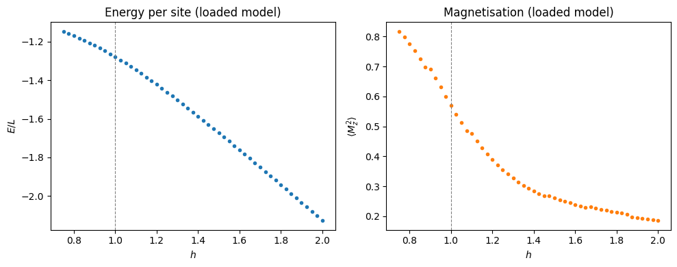
Post-training analysis#
The log.log file contains the full training history as a plain JSON dictionary.
After plotting convergence we use the loaded model to compute an IS-based
energy and magnetisation sweep — the same procedure as in Tutorial 1, but
starting from a saved checkpoint rather than a freshly trained model.
with open(os.path.join(run_dir, "log.log")) as f:
    log_data = json.load(f)

iters  = np.array(log_data["Mean Energy"]["iters"])
E_mean = np.array(log_data["Mean Energy"]["Mean"])

fig, ax = plt.subplots(figsize=(7, 3))
ax.plot(iters, E_mean / L_r)
ax.set_xlabel("Iteration")
ax.set_ylabel("$E / L$")
ax.set_title("Energy convergence (mean over replicas)")
plt.tight_layout()
plt.show()
Mz  = sum(nkf.operator.sigmaz(hi_r, i) for i in range(L_r)) * (1.0 / L_r)
Mz2 = Mz @ Mz

h_anchors = np.linspace(meta["h_min"] + 0.05, meta["h_max"] - 0.05, 7)
h_sweep   = np.linspace(meta["h_min"], meta["h_max"], 51)

# Thermalise each anchor (MCMC until R-hat < rhat_tol) before using it as an
# IS reference — see Tutorial 3 for why un-thermalised references bias the sweep.
anchor_states = {}
for h0 in h_anchors:
    mc = vs_r.get_state(jnp.array([h0]))
    mc.n_samples = 4096
    mc.thermalise(create_operator_r(jnp.array([h0])), rhat_tol=1.03, verbose=False)
    anchor_states[h0] = mc

def nearest(h):
    return h_anchors[np.argmin(np.abs(h_anchors - h))]

is_E, is_Mz2 = [], []
for h0 in h_sweep:
    mc_ref = anchor_states[nearest(h0)]
    pars   = jnp.array([h0])
    # ISState caches weights; both .expect() calls below reuse them.
    is_st  = ISState.from_mc_state(mc_ref, pars)
    op     = create_operator_r(pars)
    is_E.append(float(is_st.expect(op).mean.real))
    is_Mz2.append(float(is_st.expect(Mz2).mean.real))

is_E, is_Mz2 = np.array(is_E), np.array(is_Mz2)

fig, axes = plt.subplots(1, 2, figsize=(10, 4))

axes[0].plot(h_sweep, is_E / L_r, "o", ms=3, color="tab:blue")
axes[0].axvline(1.0, ls="--", color="gray", lw=0.8)
axes[0].set_xlabel("$h$")
axes[0].set_ylabel("$E / L$")
axes[0].set_title("Energy per site (loaded model)")

axes[1].plot(h_sweep, is_Mz2, "o", ms=3, color="tab:orange")
axes[1].axvline(1.0, ls="--", color="gray", lw=0.8)
axes[1].set_xlabel("$h$")
axes[1].set_ylabel(r"$\langle M_z^2 \rangle$")
axes[1].set_title("Magnetisation (loaded model)")

plt.tight_layout()
plt.show()